Allocation by Priority

Vensim includes built-in allocation functions that solve problems that can be impossible to handle realistically in simpler languages, and where mechanisms common in economics fail important reality checks.

In business and economic models, there is often a need to represent the allocation of a possibly-limited supply to a number of demand entities. It is also often desirable to represent the allocation of a demand among competing suppliers. Although the two kinds of problems, demand allocation and supply allocation, seem to be different, they can be effectively solved by a single algorithm. In each case, the inputs are:

• a vector of demands
• a vector of priorities
• a supply, to be allocated across the demands

In a different guise, the same problem has the following inputs

• a vector of supply capacities
• a vector of attractivenesses of the various suppliers
• a demand, to be distributed across the suppliers

In some problems, both might be present, requiring an allocation of a commodity from many demanders to many suppliers.

The ALLOCATION BY PRIORITY function (or the ALLOC P function is used in conjunction with the MARKETP function) finds a market priority at which the market clears and uses this to determine allocations.

Formulations based only on us/(us+them) logic or aggregate production functions often fail important reality checks. Vensim’s allocation functions bring some additional refinements to the allocation problem, while remaining computationally fast and simple.

General strategy: avoid doing something stupid

There are several standard approaches to modeling allocation, but each formulation has at least one important flaw. For example, one approach is to assign to each supplier a fraction ‘f’ of the demand, according to the simple formula:

f_i = (a_i / sum(a_i)) * demand

where

f_i = fraction of demand won by supplier i (in other words, supplier i’s market share)

a_i = attractiveness of supplier i’s offering (if price were the only difference among the products, a_i might be 1/price_i)

sum(a_i) is the sum of all the attractivenesses.

This formula has many desirable properties, but it fails one constraint: it is possible for a tiny supplier to capture the entire market. For example, suppose the demand is the total global demand for word-processing software. Suppose, further that there are only two competitors: Microsoft, and JoeBob’s. Microsoft is a world-wide giant; JoeBob’s is two teenage brothers (Joe and Bob) operating out of their parents’ kitchen. If Joe and Bob manage to write a better (more attractive) product than Microsoft (it’s been done before — remember Intuit), then the above formula will immediately award a majority of the market to JoeBob’s.

We can overcome this problem in two ways. One would be to include measures of visibility in the attractiveness number. In that case, JoeBob’s product might be best, but its attractiveness would be tiny, because of lack of word-of-mouth and advertising. But what if they get some rapid publicity from a review in a magazine? To do this right, we’d have to include in the attractiveness the effect of JoeBob’s overloaded telephones, etc.

As this example suggests, the allocation problem turns out to be trickier than it seems.

Requirements of a realistic allocation logic

The ALLOC P function was invented by William T. Wood in response to the challenge to find an algorithm that meets all the desired properties. There are five desired properties, to ensure both realism and flexibility:

• Deliveries to the receiving sectors must sum to the amount delivered from the supplying sector, under all conditions.
• All deliveries (allocations) must be positive.
• No sector should receive more than it orders.
• Under conditions of adequate supply, each sector should receive exactly what it orders.
• Under conditions of shortages, uniquely low-priority sectors should receive very little or nothing; if there is a uniquely high-priority sector with high demand, it should receive virtually everything, shutting out its competitors.

Phrased in the dual scheme of market shares, the same five requirements are:

• Sales of all the suppliers must sum to the total demand, under all conditions.
• All sales and market shares must be positive.
• No supplier can sell more than its capacity.
• Under conditions of extreme excess demand, each supplier should sell its entire capacity.
• Under conditions of limited demand, uniquely unattractive suppliers should sell little or nothing. If there is a uniquely attractive supplier with high capacity, it should win virtually the entire market, shutting out its competitors.

The Wood algorithm: example application

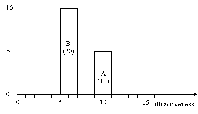
The Wood algorithm is geometrical in its inspiration, so it is best understood pictorially, in a sort of graph. Suppose there are two suppliers, A and B, with capacities of 10 and 20 widgets. We represent each supplier’s capacity by a rectangle, so the graph resembles a bar graph, except that each supplier’s capacity is represented by the area of its rectangle, not the height. The reason for using area instead of height will become apparent in a moment.

For our first example, we start with rectangles of width 2 attractiveness units. As we said, the height of each supplier’s rectangle is chosen to make the area of the rectangle equal to the capacity of the supplier. Supplier A has capacity of 10, so its rectangle’s height is 10/2, or 5 distribution units per attractiveness unit. Supplier B has a capacity of 20, so its height is 10. The center of each supplier’s rectangle is placed on the X-axis at the attractiveness value of the supplier’s offering: the more attractive suppliers (independent of their supply capacity) are placed to the right. Suppliers A and B have attractivenesses of 10 and 6, respectively, so their rectangles are placed on the attractiveness axis as shown in Figure 1.

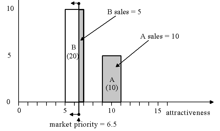
Suppose that suppliers A and B, as shown in Figure 1, are competing for a market of 15 widgets. The Wood algorithm represents the market as a vertical line that moves in from the right, as shown in Figure 2. The market line continues to move until it has swept out an area equal to the total market, and then it stops. In Figure 2, the line has swept out an area of 15 widgets (the shaded region in Figure 2) and has stopped at attractiveness value 6.5. The attractiveness value at which it stops is the “market priority,” or the attractiveness which clears the market. If the capacities of the suppliers are insufficient to cover the market, then each supplier sells all of its capacity.

Because our first example uses a width parameter (2), less than the gap in attractiveness between suppliers A and B, the algorithm enforces a kind of “first come, first serve” allocation. The width parameter is simply the difference in attractiveness it takes to achieve exclusive first rights over a competitor (up to one’s capacity, of course). The following example shows the effect of an increased width parameter.

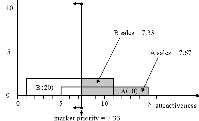
Figure 3 shows the same example, but with the width parameter set to 10. The market line has come in from the right, as always, and as it encounters the right edge of supplier A, it sweeps out 1 widget for each unit of attractiveness. By the time it reaches the right edge of supplier B, it has allocated 4 widgets to supplier A. In the region of attractiveness where A and B overlap, each unit of attractiveness covers 2 widgets from B and 1 from A. The total number of widgets allocated reaches 15 when the market line reaches attractiveness of 7.33, as shown at the bottom of Figure 3

As suggested by the above two examples, the Wood algorithm meets all of the five requirements. We are aware of no other algorithm that conforms to all five. In addition, the Wood algorithm is flexible enough to serve as a realistic model of most allocation and market competition situations.

Implementation in Vensim

Vensim uses the ALLOCATION BY PRIORITY function to allocate resources with this algorithm.

First you create a variable (e.g., mp) to hold the market priority then enter the arguments of the MARKETP function:

allocation[subscript] = AllOCATE BY PRIORITY(
request[subscript],
priority[subscript],
size,
width,
supply)

Request is the amount desired by the entities. Priority is the priority given to the entities. Size is the number of entities (normally this is just ELMCOUNT(subscript). Width is the measure of the size of attractiveness (see above). Supply is the total supply to be divided (a single value from a variable).

Multiple Subscripts

If you have variables with more than one subscript you must use the subscript over which allocation is being made last. Suppose, for example, you are allocating market share to different companies by state. You might have:

sales[state,company] = ALLOCATE BY PRIORITY(
capacity[state,company],
attractiveness[state,company],
ELMCOUNT(company),
attractiveness width[state],
total demand[state])