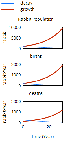
Next, we will make changes to a model Constant to generate exponential decay or decline in the population. Like exponential growth, this is one of the simplest possible dynamic behaviors.
| Ø | Double click on the run name and replace growth with decay. |
Do one of:
| Ø | Click on the SyntheSim button. |
| Ø | Drag the Slider under average lifetime till it displays a value of 4. |
| Ø | Click on the Stop Button |
Or
| Ø | Click on the Set Up a Simulation button. |
| Ø | Click on the variable average lifetime (appearing blue/yellow in the sketch) and in the editing box type the value 4. Press the Enter key. |
| Ø | Click the Simulate button and the model will simulate. |
Both the above sets of steps result in the creation of the new run decay.
| Ø | Click on the Graph tool and compare the three runs. |
| Ø | Click on the Control Panel button on the Main Toolbar. In the Datasets Control box, double click on the run equilib in the right box; this will unload the run so the Analysis tools will not examine it. Note that it can be reloaded just as easily. (You can also single click to select the run then use the Move button (<<) or (>>) to unload or load the dataset.) |
| Ø | Click on the Causes Strip tool; a strip graph is generated showing Population and its causes — births and deaths, for the two last runs. |

Population declines in the decay run because the average lifetime was set to a lower value than the equilibrium value. This made the negative feedback loop through deaths stronger than the positive feedback loop through births, resulting in Population decline over time.
