Optimization
Vensim’s optimizer provides fast calibration of models and discovery of optimal solutions
Model Calibration
Validation of the integrity of a model rests in part on comparing model behavior to time series data collected in the “real world.” When a model is structurally complete and simulates properly, calibration of the model can proceed to fit the model to this observed data. Dynamic models are often very sensitive to the values of constant parameters. If you want to calibrate your parameters so the model behavior matches observed data, you may need to experiment with thousands of combinations of different parameter values. Vensim calibration makes this procedure automatic. You specify which data series you want to fit and which parameters you want to adjust, then Vensim automatically adjust parameters to get the best match between model behavior and the data. There are no limits on the numbers of parameters to adjust or data series to fit.
Example
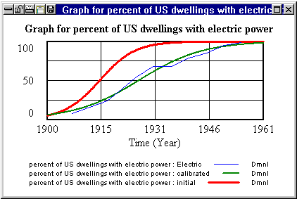
Over the last century, the conversion of U.S. households to electricity follows a pattern of diffusion, represented by a Bass Diffusion model. Once the structure is complete and produces the desired behavior patterns, we can calibrate the model to fit historical data from the U.S. Department of Commerce. The first simulation run (first run) shows growth too early and too fast compared to the historical data (historical). The user selects the parameters that have unknown or uncertain values and selects the data series historical, then the Vensim optimization engine searches for the values of the parameters that gives the best fit to the data, and displays the values of the parameters and the best simulation run (calibrated).
Policy Optimization
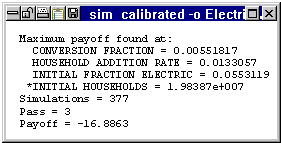
Vensim’s optimizing engine can search through a large space of parameter values looking for optimal solutions. You define the payoff variables you want to adjust. An efficient Powell hill climbing algorithm searches through the parameter space looking for the largest cumulative payoff. There are no limits on the numbers of payoff variables or policy parameters to search over. Advanced sensitivity analysis is available from optimization simulations.
Example
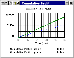
A company features an inventory and sales supply chain which it must manage to maximize company profits. Too little inventory leads to loss of sales (and lower profits) but too much inventory costs more to stock and also leads to lower profits. The user selects the payoff variables, in this case Cumulative Profit, and then selects the policy parameters (minimum inventory value to start restocking, and maximum inventory value to stop restocking). The Vensim optimization engine searches for the values of the policy parameters that gives the best payoff value (highest Cumulative Profit) and prints out the values and the optimal simulation run.
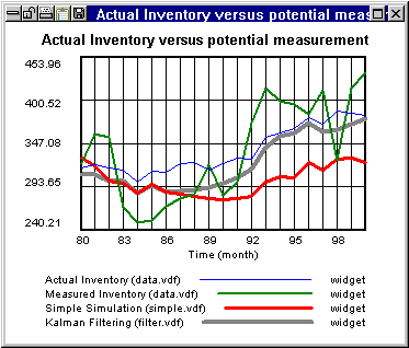
Kalman Filtering
In a dynamic system with unobserved variables it is desirable, but impossible to know, the state of all variables at all times. However, if values for some of the variables are known, you can make a good estimate of the values of other variables. For example, a business model might consist of a Workforce/Inventory system. The goal is to determine the time profiles of workforce, inventory, and other model variables given the available measurements. Vensim simulates the model with the Kalman filter active and makes intelligent choices for the output, based on both the model Simple Simulation data (simple.vdf in graph below) and Measured Inventory data (data.vdf). The resulting output Kalman Filtering (filter.vdf – grey line) tracks the Actual Inventory (blue line) much better than either the simple simulation alone (red line) or the measured inventory alone (green line).