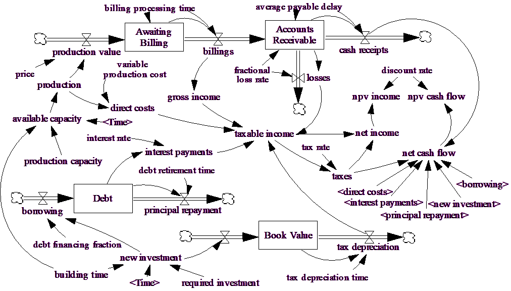
The remainder of the model is quite straightforward to construct. Usually, the most difficult issues involve representation of the tax system faced by the corporation. We have opted for a simple proportional tax that would be appropriate in many situations. We have also used proportional depreciation of book value for tax purposes and proportional debt retirement. These formulations were chosen because of their simplicity.

We have added in two additional Levels — Debt and Book Value. If you look for feedback in this model you will find only the short draining loops around each Level. This is a dynamically simple model with a reasonably high amount of detail around the cash flow and taxable income. The way the model is set up required investment occurs over building time and then production comes on line at capacity. The model, as constructed, is for a fixed up front investment followed by a realized cash flow from production.
The model uses the NPV function to compute a net present value for both income and cash flow. The NPV function is a dynamic function that takes as arguments a stream of payments, a discount rate, an initial value and an adjustment factor. We are using 0 as an initial value and 1 as the adjustment factor. With these argument the NPV will, at the end of the simulation, report the present value of the stream as of the beginning of the simulation.
Model Equations
| Book Value = INTEG( |
| new investment - tax depreciation, |
| 0) |
Units: $
tax depreciation = Book Value / tax depreciation time
Units: $/Year
| taxable income = gross income - direct costs - losses - |
| interest payments - tax depreciation |
Units: $/Year
production = available capacity
Units: Widget/Year
| available capacity = IF THEN ELSE ( Time >= building time, |
| production capacity, 0) |
Units: Widget/Year
tax depreciation time = 10
Units: Year
tax rate = 0.4
Units: Dmnl
| Accounts Receivable = INTEG( |
| billings - cash receipts - losses, |
| billings/(1/average payable delay + fractional loss rate)) |
Units: $
average payable delay = 0.09
Units: Year
| Awaiting Billing = INTEG( |
| price * production - billings, |
| price * production * billing processing time) |
Units: $
billing processing time = 0.04
Units: Year
billings = Awaiting Billing / billing processing time
Units: $/Year
borrowing = new investment * debt financing fraction
Units: $/Year
building time = 1
Units: Year
cash receipts = Accounts Receivable / average payable delay
Units: $/Year
| Debt = INTEG( |
| borrowing - principal repayment, |
| 0) |
Units: $
debt financing fraction = 0.6
Units: Dmnl
debt retirement time = 3
Units: Year
direct costs = production * variable production cost
Units: $/Year
discount rate = 0.12
Units: 1/Year
fractional loss rate = 0.06
Units: 1/Year
gross income = billings
Units: $/Year
interest payments = Debt * interest rate
Units: $/Year
interest rate = 0.12
Units: 1/Year
losses = Accounts Receivable * fractional loss rate
Units: $/Year
| net cash flow = cash receipts + borrowing - new investment - |
| direct costs - interest payments - principal repayment - taxes |
Units: $/Year
net income = taxable income - taxes
Units: $/Year
| new investment = IF THEN ELSE (Time >= building time, 0, |
| required investment / building time) |
Units: $/Year
npv cash flow = NPV (net cash flow, discount rate, 0, 1)
Units: $
npv income = NPV (net income, discount rate, 0, 1)
Units: $
PRICE = 1
Units: $/Widget
principal repayment = Debt / debt retirement time
Units: $/Year
production capacity = 2400
Units: Widget/Year
required investment = 2000
Units: $
taxes = taxable income * tax rate
Units: $/Year
variable production cost = 0.6
Units: $/Widget
TIME STEP = 0.015625
Simulation Results
We run the model for 5 years with TIME STEP = 0.015625.

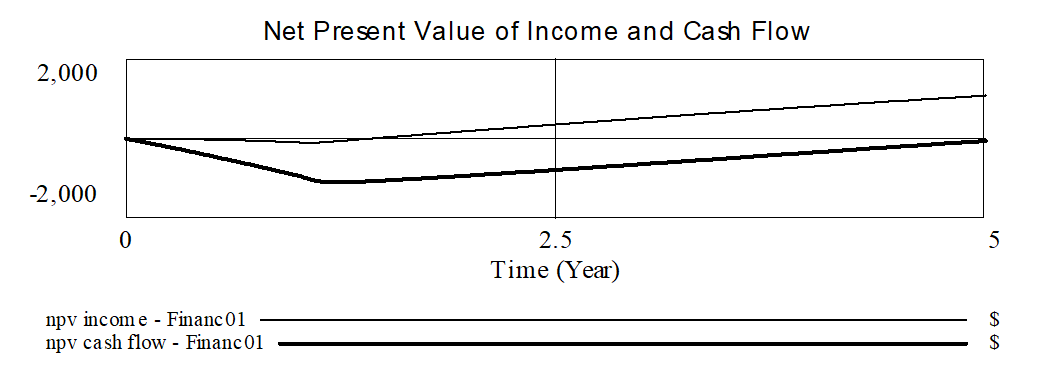
At the end of the simulation npv income is $1,073 while npv cash flow is -$54.70 (this is on a total investment of $2,000. If we plot the present values over the course of the simulation we get:

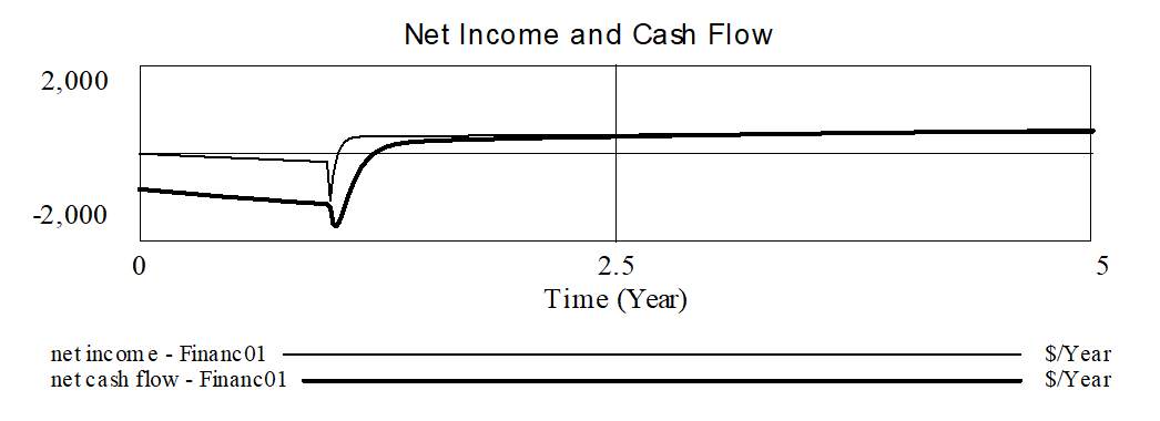
There is a significant difference between the income and cash flow profiles — and this is a result of the manner in which income is computed.