To best illustrate what the Kalman filter does and how it can be used, an example is useful. This example is based on the workforce inventory model wfkal.mdl in the directory \models\sample\kalman.
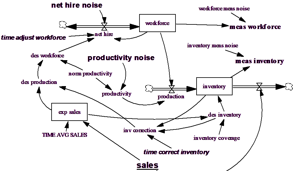
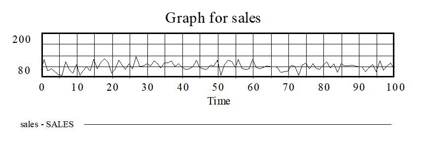
The two measurements on the system are meas workforce and meas inventory. Both of these are direct measurements containing errors (meas noise) from for the corresponding model levels. Sales is an exogenous driver, with values specified in the data file sales.dat.
Noise that drives model behavior enters the system through net hire noise and productivity noise.
The goal is to determine the time profiles of workforce, inventory and the other model variables given the available measurements. One approach to this problem would be to assume that workforce and inventory are equal to their measured values. Another would be to simulate the model with productivity noise and net hire noise both set to 0. The first of these approaches uses only the data, the second only the model. Kalman filtering provides a mechanism to intelligently combine the data and model in making indirect measurements of the model variables.
Creating the "Data"
To illustrate the purpose and value of Kalman filtering we will use the model to generate "data." This technique allows us to easily review the unobservable variables (the time profiles of workforce, inventory and other variables) and see how they simulate relative to what actually happens. To create this data:
Import the data file sales.dat and enter this dataset (sales.vdf) into the Data Sources field in the Advanced tab of the Simulation Control.
Select the Changes tab of the Simulation Control, click the Load Changes from… button and open the file wfkal_n.cin containing:
productivity_noise = .20
workforce meas noise = .025
inventory meas_noise = 0.1
net hire noise = 4
Enter the run name data and simulate the model. We will use this run (data.vdf) as though it were data collected from the real world.
Setting up the Filter
The Kalman filter requires the specification of the driving noise variance and the measurement error variance. The function RANDOM UNIFORM(-.5,.5,0) returns a random variable with a mean of 0 and a variance of .08333. We multiply this times the random input magnitude assumed in making the constant changes squared. Specifically:
meas inventory variance = 55 { .0833 * (.1*300)2 }
meas workforce variance = .5 { .0833 *( 0.025*100)2 }
inventory drive variance = 33 {0833*(.2*1*100)2 }
workforce drive variance = 1.3 {.0833*(4)2 }
Note that both the net hire error and the productivity error integrate directly into the levels and that TIME STEP is 1 in this model.
The above values are set in the model to help define the Kalman filter. The first two values are used in the payoff file (wfkal.vpd) as:
*Calibration
MEAS_WORKFORCE/MEAS_WORKFORCE_VARIANCE
MEAS_INVENTORY/MEAS_INVENTORY_VARIANCE
The second two values are used to define the driving noise covariance in the Kalman filter file kalman.prm as:
inventory/inventory drive_variance/.1
workforce/workforce drive variance/.1
Here we have set the initial state covariance to a small number for each state variable. The Kalman filter file (kalman.prm) must be created in the Text Editor (or you can use the existing file for this example).
Simulating
We will make two simulations. The first called simple.vdf will simulate the model with no filtering. The second called filter.vdf will simulate the model with Kalman filtering active.
Remove the changes file wfkal_n.cin from the Load Changes from… field in the Changes Tab (or you will be simulating what you have already simulated).
Enter the run name simple and click the Simulate button to simulate the model.
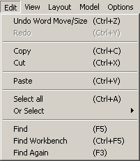
For the Kalman filtering run, enter the run name filter. Enter the real world data (data.vdf) into the Data Sources… field (along with sales.vdf). Enter the payoff file wfkal.vpd in the Payoff Definition… field. Turn on Kalman filtering by checking the Kalman Filtering box. When you click on this the file kalman.prm will automatically be used. You do not need to name this file in the Simulation Control dialog. The Simulation Control should appear as below:
Click the Simulate button to simulate the model with Kalman filtering.
You can now compare the two alternative ways of measuring inventory and workforce (simple simulation and simulation with Kalman filtering). The custom graph named COMPARE will do this.

Though each method is in the ball park, simple simulation is not tracking very well. Blowing up the last 20 months shows:
The use of filtering provides better estimates of the amount of inventory by combining the information in the model (that predicts what a value will be) with the information in the measurements (data collected from the system). This is true for measured variables, and it is also true for unmeasured variables. For example, suppose that we had measurements for Workforce but not for Inventory. It is still possible to make estimates of the value of Inventory using this data. If you create the file wfkal2.vpd containing:
*Calibration
MEAS_WORKFORCE/MEAS_WORKFORCE_VARIANCE
And simulate the model naming the run filter2. You will get the estimate of inventory (using the Graph Compare2) as:
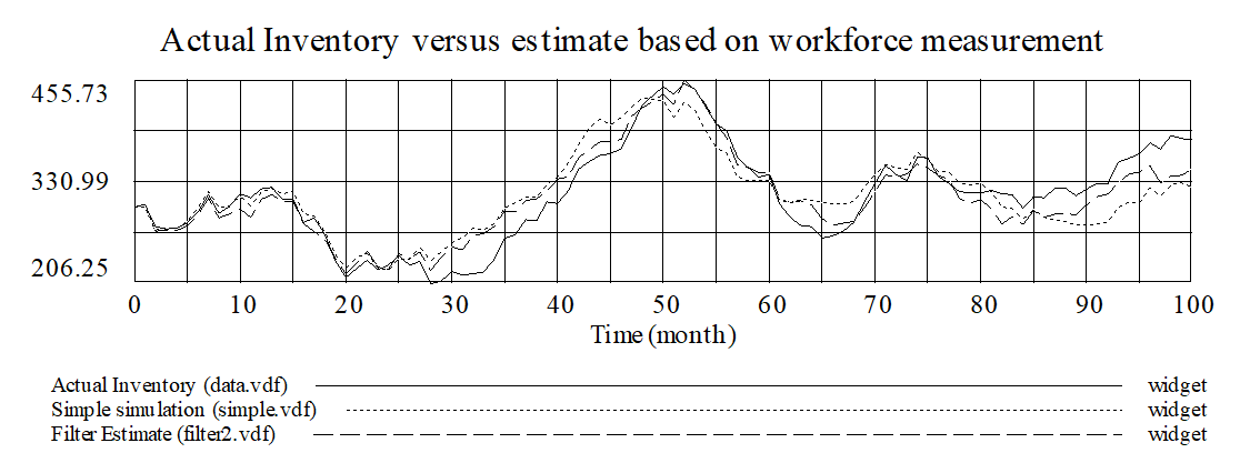
This is somewhat less accurate than what was obtained with measurements on Inventory.But it is remarkable that having measurements only on Workforce allows a reasonably good estimate of the values of Inventory in a noisy system.
The addition of the Kalman filter provides an ability to recover reasonable estimates of the underlying dynamics (the time profiles of workforce and inventory). This is potentially valuable for any model, and is critical for a model that contains unobserved dynamics of a transient nature.