Before we get started on the discrete examples it is useful to see the continuum that exists between discrete and continuous models. This is most vividly displayed by looking at a model that has several types of delays ModelGuide\9discret\discon.mdl..

In this model outflow 1 is the outflow of a first order delay, outflow 3 a third order delay, outflow n and nth order delay (n is a model constant) and outflow discrete a discrete or infinite order delay. The order of a delay is determined by the number of levels involved in the delay. For the first and third order delays this number is obvious. For the nth order and discrete delays the number of levels is hidden in the internal structures used to compute the equations.
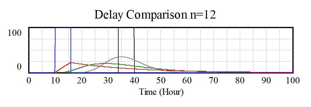
Now look at the behavior of this model when n is 12:

and when n is 100

It is useful to experiment with this model, though it does become slow to simulate with large values for n. The key thing to observe is that as n increases we get closer and closer to a discrete delay, but never actually get there. Even with a 100th order delay there is a noticeable difference, though if you compare Accumulation N and Accumulation Discrete they are not much different.
As a note, for the discrete delay the number of levels is not really infinite, it is actually equal to processing time/TIME STEP. The output of the high order delay functions, such as DELAY FIXED and DELAY N, are held constant across each TIME STEP. This allows alternative integration techniques to be mixed with discrete delays in a sensible manner.